New improved Australia RSS TLT satellite temperature

In my first attempt at this I got the longitude wrong (details here). Having corrected that, in my second attempt I defined a smaller rectangle to avoid any ocean areas as shown in the graph that follows.



...which yields the graph (16-point moving average in red):




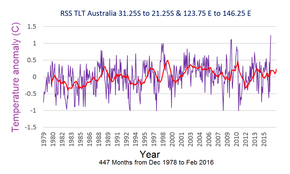
In the end I decided the ocean areas didn't affect things that much because the larger area was a better match to Steve Goddard's graph of 25 randomly chosen points.  So I prefer the one below. Here is the map area measured:



And here is my derived anomaly with 12-point moving average to match Goddard's with Matlab code:

a1 =
ncread('uat4_tb_v03r03_anom_chtlt_197812_201602.nc3.nc','brightness_temperature_anomaly')
AusNew = squeeze(tsnansum(a1(118:131,:,:)))
AusNew2 = squeeze(tsnansum(AusNew(23:30,:)))
Aus3=AusNew2'
Aus4 = Aus3/(8*14)
plot(Aus4)

Here is the Steven Goddard graph:



Here is the official up-tweaked BoM version which note extends further back in time (from here):